Is heavy physical activity a major trigger of death by sudden cardiac arrest? Not in Oregon

The idea that heavy physical activity is a main trigger of heart attacks is widespread. Often endurance running and cardio-type activities are singled out. Some people refer to this as “death by running”.

Good cardiology textbooks, such as the Mayo Clinic Cardiology, tend to give us a more complex and complete picture. So do medical research articles that report on studies of heart attacks based on comprehensive surveys.

Reddy and colleagues (2009) studied sudden cardiac arrest events followed by death from 2002 to 2005 in Multnomah County in Oregon. This study was part of the ongoing Oregon Sudden Unexpected Death Study. Multnomah County has an area of 435 square miles, and had a population of over 677 thousand at the time of the study. The full reference to the article and a link to a full-text version are at the end of this post.

The researchers grouped deaths by sudden cardiac arrests (SCAs) according to the main type of activity being performed before the event. Below is how the authors defined the activities, quoted verbatim from the article. MET is a measure of the amount of energy spent in the activity; one MET is the amount of energy spent by a person sitting quietly.

- Sleep (MET 0.9): subjects who were sleeping when they sustained SCA.
- Light activity (MET 1.0–3.4): included bathing, dressing, cooking, cleaning, feeding, household walking and driving.
- Moderate activity (MET 3.5–5.9): included walking for exercise, mowing lawn, gardening, working in the yard, dancing.
- Heavy activity (MET score ≥6): included sports such as tennis, running, jogging, treadmill, skiing, biking.
- Sexual activity (MET score 1.3): included acts of sexual intercourse.

What did they find? Not what many people would expect.

The vast majority of the people dying of sudden cardiac arrest were doing things that fit the “light activity” group above prior to their death. This applies to both genders. The figure below (click to enlarge) shows the percentages of men and women who died from sudden cardiac arrest, grouped by activity type.

Sudden cardiac arrests were also categorized as witnessed or un-witnessed. For witnessed, someone saw them happening. For un-witnessed, the person was seen alive, and within 24 hours had died. So the data for witnessed sudden cardiac arrests is a bit more reliable. The table below displays the distribution of mean age, gender and known coronary artery disease (CAD) in those with witnessed sudden cardiac arrest.

Look at the bottom row, showing those with known coronary artery disease. Again, light activity is the main trigger. Sleep comes second. The numbers within parentheses refer to percentages within each activity group. Those percentages are not very helpful in the identification of the most important triggers, although they do suggest that coronary artery disease is a major risk factor. For example, among those who died from sudden cardiac arrest while having sex, 57 percent had known coronary artery disease. For light activity, 36 percent had known coronary artery disease.

As a caveat, it is worth noting that heavy activity appears to be more of a trigger in younger individuals than in older ones. This may simply reflect the patterns of activities at different ages. However, this does not seem to properly account for the large differences observed in triggers; the standard deviation for age in the heavy activity group was large enough to include plenty of seniors. Still, it would have been nice to see a multivariate analysis controlling for various effects, including age.

So what is going on here?

The authors give us a hint. The real culprit may be bottled up emotional stress and sleep disorders; the latter may be caused by stress, as well as by obesity and other related problems. They have some data that points in those directions. That makes some sense.

We humans have evolved “fight-or-flight” mechanisms that involve large hormonal discharges in response to stressors. Our ancestors needed those. For example, they needed those to either fight or run for their lives in response to animal attacks.

Modern humans experience too many stressors while sitting down, as in stressful car commutes and nasty online interactions. The stresses cause “fight-or-flight” hormonal discharges, but are followed by neither “fight” nor “flight” in most cases. This cannot be very good for us.

Death by running!? More like death by not running!

Reference:

Reddy, P.R., Reinier, K., Singh, T., Mariani, R., Gunson, K., Jui, J., & Chugh, S.S. (2009). Physical activity as a trigger of sudden cardiac arrest: The Oregon Sudden Unexpected Death Study. International Journal of Cardiology, 131(3), 345–349.

Long distance running causes heart disease, unless it doesn’t

Regardless of type of exercise, disease markers are generally associated with intensity of exertion over time. This association follows a J-curve pattern. Do too little of it, and you have more disease; do too much, and incidence of disease goes up. There is always an optimal point, for each type of exercise and marker. A J curve is actually a U curve, with a shortened left end. The reason for the shortened left end is that, when measurements are taken, usually more measures fall on the right side of the curve than on the left.

The figure below (click to enlarge) shows a schematic representation that illustrates this type of relationship. (I am not very good at drawing.) Different individuals have different curves. If the vertical axis was a measure of health, as opposed to disease, then the curve would have the shape of an inverted J.

The idea that long distance running causes heart disease has been around for a while. Is it correct?

If it is, then one would expect to see certain things. For example, let’s say you take a group of long distance runners who have been doing that for a while, ideally runners above age 50. That is when heart disease becomes more frequent. This would also capture more experienced runners, with enough running experience to cause some serious damage. Let us say you measured markers of heart disease before and after a grueling long distance race. What would you see?

If long distance running causes heart disease, you would see a significant proportion with elevated makers of heart disease among the runners at baseline (i.e., before the race). After all, running is causing a cumulative problem. The levels of those markers would be correlated with practice, or participation in previous races, since the races are causing the damage. Also, you would see a uniformly bad increase in the markers after the race, as the running is messing up everybody more or less equally.

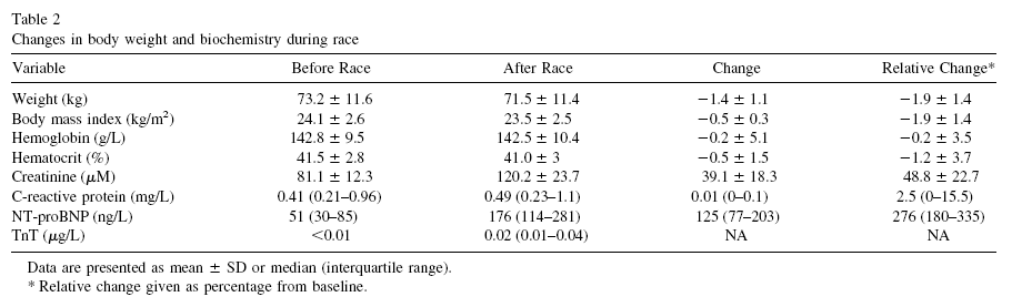
Sahlén and colleagues (2009), a group of Swedish researchers, studied males and females aged 55 or older who participated in a 30-km (about 19-mile) cross-country race. The full reference to the article is at the end of this post. The researchers included only runners who had no diagnosed medical disorders in their study. They collected data on the patterns of exercise prior to the race, and participation in previous races. Blood was taken before and after the race, and several measurements were obtained, including measurements of two possible heart disease markers: N-terminal pro-brain natriuretic peptide (NT-proBNP), and troponin T (TnT). The table below (click to enlarge) shows several of those measurements before and after the race.

We can see that NT-proBNP and TnT increased significantly after the race. So did creatinine, a byproduct of breakdown in muscle tissue of creatine phosphate; something that you would expect after such a grueling race. Yep, long distance running increases NT-proBNP and TnT, so it leads to heart disease, right?

Wait, not so fast!

NT-proBNP and TnT levels usually increase after endurance exercise, something that is noted by the authors in their literature review. But those levels do not stay elevated for too long after the race. Being permanently elevated, that is a sign of a problem. Also, excessive elevation during the race is also a sign of a potential problem.

Now, here is something interesting. Look at the table below, showing the variations grouped by past participation in races.

The increases in NT-proBNP and TnT are generally lower in those individuals that participated in 3 to 13 races in the past. They are higher for the inexperienced runners, and, in the case of NT-proBNP, particularly for those with 14 or more races under their belt (the last group on the right). The baseline NT-proBNP is also significantly higher for that group. They were older too, but not by much.

Can you see a possible J-curve pattern?

Now look at this table below, which shows the results of a multiple regression analysis on its right side. Look at the last column on the right, the beta coefficients. They are all significant, but the first is .81, which is quite high for a standardized partial regression coefficient. It refers to an almost perfect relationship between the log of NT-proBNP increase and the log of baseline NT-proBNP. (The log transformations reflect the nonlinear relationships between NT-proBNP, a fairly sensitive health marker, and the other variables.)

In a multiple regression analysis, the effect of each independent variable (i.e., each predictor) on the dependent variable (the log of NT-proBNP increase) is calculated controlling for the effects of all the other independent variables on the dependent variable. Thus, what the table above is telling us is that baseline NT-proBNP predicts NT-proBNP increase almost perfectly, even when we control for age, creatinine increase, and race duration (i.e., amount of time a person takes to complete the race).

Again, even when we control for: AGE, creatinine increase, and RACE DURATION.

In order words, baseline NT-proBNP is what really matters; not even age makes that much of a difference. But baseline NT-proBNP is NEGATIVELY correlated with number of previous races. The only exception is the group that participated in 14 or more previous races. Maybe that was too much for them.

Okay, one more table. This one, included below, shows regression analyses between a few predictors and the main dependent variable, which in this case is TnT elevation. No surprises here based on the discussion so far. Look at the left part, the column labeled as “B”. Those are correlation coefficients, varying from -1 to 1. Which is the predictor with the highest absolute correlation with TnT elevation? It is number of previous races, but the correlation is, again, NEGATIVE.

In follow-up tests after the race, 9 out of the 185 participants (4.9 percent) showed more decisive evidence of heart disease. One of those died while training a few months after the race. An autopsy was conducted showing abnormal left ventricular hypertrophy with myocardial fibrosis, coronary artery narrowing, and an old myocardial scar.

Who were the 9 lucky ones? You guessed it. Those were the ones who had the largest increases in NT-proBNP during the race. And large increases in NT-proBNP were more common among the runners who were too inexperienced or too experienced. The ones at the extremes.

So, here is a summary of what this study is telling us:

- The 30-km cross-country race studied is no doubt a strenuous activity. So if you have not exercised in years, perhaps you should not start with this kind of race.

- By and large, individuals who had elevated markers of heart disease prior to the race also had the highest elevations of those markers after the race.

- Participation in past races was generally protective, likely due to compensatory body adaptations, with the exception of those who did too much of that.

- Prevalence of heart disease among the runners was measured at 4.9 percent. This does not beat even the mildly westernized Inuit, but certainly does not look so bad considering that the general prevalence of ischemic heart disease in the US and Sweden is about 6.8 percent.

It seems reasonable to conclude that long distance running may be healthy, unless one does too much of it. The ubiquitous J-curve pattern again.

How much is too much? It certainly depends on each person’s particular health condition, but the bar seems to be somewhat high on average: participation in 14 or more previous 30-km races.

As for the 4.9 percent prevalence of heart disease among runners, maybe it is caused by something else, and endurance running may actually be protective, as long as it is not taken to extremes. Maybe that something else is a diet rich in refined carbohydrates and sugars, or psychological stress caused by modern life, or a combination of both.

Just for the record, I don’t do endurance running. I like walking, sprinting, moderate resistance training, and also a variety of light aerobic activities that involve some play. This is just a personal choice; nothing against endurance running.

Mark Sisson was an accomplished endurance runner; now he does not like it very much. (Click here to check his excellent book The Primal Blueprint). Arthur De Vany is not a big fan of endurance running either.

Still, maybe the Tarahumara and hunter-gatherer groups who practice persistence hunting are not such huge exceptions among humans after all.

Reference:

Sahlén, A., Gustafsson, T.P., Svensson, J.E., Marklund, T., Winter, R., Linde, C., & Braunschweig, F. (2009). Predisposing Factors and Consequences of Elevated Biomarker Levels in Long-Distance Runners Aged >55 Years. The American Journal of Cardiology, 104(10), 1434–1440.

Healthy Spirits: Fantome and More!!!

Some great stuff today!

1. Fantome
2. Fantome Dark White
3. Fantome Chocolat
4.Augustijn Ale
5. Augustiner-Brau Edelstoff and Maximator are back!!!


cheers,

dave hauslein
beer manager
415-255-0610

Niacin and its effects on growth hormone, glucagon, cortisol, blood lipids, mental disorders, and fasting glucose levels

Niacin is a very interesting vitamin. It is also known as vitamin B3, or nicotinic acid. It is an essential vitamin whose deficiency leads to a dreadful disease known as pellagra. In large doses of 1 to 3 g per day it has several effects on blood lipids, including these: it increases HDL cholesterol, decreases triglycerides, and decreases Lp(a). Given that this is essentially a reversal of the metabolic syndrome, for those who are on their way to developing it, niacin must really do something good for our body. Niacin is also a powerful antioxidant.

The lipid modification effects of niacin are so consistent across a broad spectrum of the population that some companies that commercialize niacin-based products guarantee some measure of those effects. The graphs below (click to enlarge) are from Arizona Pharmaceuticals, a company that commercializes an instant-release niacin formulation called Nialor (see: arizonapharmaceuticals.com). The graphs show the peak effects on HDL cholesterol and triglycerides at the recommended dose, which is 1.5 g per day. The company guarantees effects; not the peak effects shown, but effects that are large enough to have clinical significance.

Niacin also has been used in the treatment of various mental disorders, including schizophrenia. Its effectiveness in this domain (mental disease) is still under debate. Yet many people, including reputable mental health researchers, swear by it. Empirical research suggests beyond much doubt that niacin helps in the treatment of depression and bipolar disorder.

Abram Hoffer, a Canadian psychiatrist who died in 2009, at the age of 91, has discussed at length the many beneficial health effects of niacin. He was also a niacin user. He argued that it can even make people live longer, and be generally healthier and more active. The effect on longevity may sound far-fetched, but there is empirical data supporting this hypothesis as well. (For more, see this book.)

By the way, moderate niacin supplementation seems to increase the milk output of cows, without any effect on milk composition.

Most people dislike the sensation that is caused by niacin, the “niacin flush”. This is a temporary sensation similar to that of sunburn covering one’s full torso and face. It goes away after a few minutes. This is niacin’s main undesirable side effect at doses up to 3 g per day. Higher doses are not recommended, and can be toxic to the liver.

Nobody seems to understand very well how niacin works. This leads to some confusion. Many people think that niacin inhibits the production of VLDL, free fatty acids, and ketones; preventing the use of fat as an energy source. And it does!

So it makes you fat, right?

No, because these effects are temporary, and are followed, often after 3 to 5 hours, by a large increase in circulating growth hormone, cortisol and glucagon. These hormones are associated with (maybe they cause, maybe are caused by) a large increase in free fatty acids and ketones in circulation, but not with an increase in VLDL secretion by the liver. So ketosis is at first inhibited by niacin, and then comes in full force after a few hours.

The decreased VLDL secretion is no surprise, because VLDL is not really needed in large quantities if muscle tissues (including the heart) are being fed what they really like: free fatty acids and ketones. When VLDL particles are secreted by the liver in small numbers, they tend to be large. As they shrink in size after delivering their lipid content to muscle tissues, they become large LDL particles; too large to cross the endothelial gaps and cause plaque formation.

It is as if niacin held you back for a few hours, in terms of fat burning, and then released you with a strong push.

Since niacin does not seem to suppress the secretion of chylomicrons by the intestines, it should be taken with meals. The meals do not necessarily have to have any carbohydrates in them. If you take niacin while fasting, you may feel “funny” and somewhat weak, because of the decrease in VLDL, free fatty acids, and ketones in circulation. These, particularly the free fatty acids and ketones, are important sources of energy in the fasted state.

Given niacin’s delayed effects, it does not seem to make much sense to take slow release niacin of any kind. In fact, the form of niacin that seems to work best is the instant-release one, the one that gives you the flush. It may be a good idea to wait until 3 to 5 hours after you take it to do heavy exercise. You may feel a surge of energy 3 to 5 hours after taking it, when the delayed effects kick in.

The delayed effects of niacin on growth hormone, cortisol and glucagon are probably the reasons why people taking niacin frequently see a small increase in fasting glucose levels. This increase is usually of a few percentage points, but can be a bit higher in some people. Growth hormone, cortisol and particularly glucagon increase blood glucose levels; and the blood levels of these hormones naturally rise in the morning to get you ready for the day ahead. Niacin seems to boost that. Hence the increase in fasting blood glucose levels. This appears to be a benign effect, easily counterbalanced by niacin’s many benefits.

In spite of a possible increase in fasting glucose levels, there is no evidence that niacin increases average blood glucose levels. If it did, that would not be a good thing. In fact, it has been argued that niacin intake can be part of an effective approach to treating diabetes; Robert C. Atkins discussed this in his Vita-Nutrient Solution book.

Niacin’s effects on lipids are somewhat similar to those of low carbohydrate dieting. For example, both lead to a decrease in fasting triglycerides and an increase in HDL cholesterol. But the mechanisms by which those effects are achieved appear to be rather different.

References:

Quabbe, H.J., Trompke, M., & Luyckx, A.S. (1983). Influence of ketone body infusion on plasma growth hormone and glucagon in man. J. Clin Endocrinol Metab., 57(3):613-8.

Quabbe, H.J., Luyckx, A.S., L'age M., & Schwarz, C. (1983). Growth hormone, cortisol, and glucagon concentrations during plasma free fatty acid depression: different effects of nicotinic acid and an adenosine derivative (BM 11.189). J. Clin Endocrinol Metab., 57(2):410-4.

Schade, D.S., Woodside, W., & Eaton, R.P. (1979). The role of glucagon in the regulation of plasma lipids. Metabolism, 28(8):874-86.

Obesity protects against disease, unless you eat butter

Notes:

- This post is a joke, a weird parody of academic research, which is why it is labeled “humor” and is being filed under “Abstract humor”. In my reading of academic articles I often come across articles with a lot of problems – interpretation biases, idiotic self-citation, moronic research designs, misguided immodesty, exaggerated political correctness, fake markers of high moral standards, nonsensical quantitative analysis etc. I decided to write a short post on a fictitious study that has all of these problems (a challenge).

- I apologize for this spoiler. Some people probably like humor posts better if they do not know what they are in advance, but several others may think that reading a post like this is a waste of their time. If you are in the latter category, move on to another post! If not, here it goes …

***

New groundbreaking forthcoming research by Drs. Deth and Disis (full reference at the end of this post) shows beyond much doubt that obesity is protective against disease. The research also implicates butter as a powerful disease-promoting agent. The research is forthcoming in the journal Butter Toxicity Review.

(Sources: Topnews.us and Flickr.com)

The journal is listed as an “elite”-level journal on the website of the Society for Research on Butter and its Negative Health Effects (SRBNHE). I thank the researchers for sharing their findings with a select group of notable scholars, of which I can humbly say I am part, well in advance of its official publication. Another seminal study by the same researchers has been cited in this post.

The study followed 2,301 male participants over a period of 13.3 years. Their ages ranged from 20 to 37 years. Approximately half of them were morbidly obese, with body fat percentages of 60 or higher. That is, more than half of these individuals’ bodies were pure fat! These obese individuals were matched against an age-compatible control group of fit men with a mean body fat percentage of 9.2.

The focus of the study was on sexually transmitted diseases among individuals with high moral standards. Because of that, the researchers noted that: “A small group of individuals, who admitted to availing themselves of adult entertainment services, and/or services of a similarly immoral nature, were excluded from the study.”

Among the fit individuals, 15.7 percent contracted one or more types of sexually transmitted diseases during the 13.3-year period. Only 3.1 percent of the obese individuals contracted ANY sexually transmitted disease. This difference was statistically significant at the .001 level (i.e., very significant), even when the researchers controlled for various demographic factors.

Even more interesting were the patterns of risk-avoidance behavior observed. The vast majority of the fit individuals (84.3 percent, to be more precise) reported using protective items (i.e., condoms). However, NONE of the obese individuals used those. And yet, the obese individuals had significantly less incidence of sexually transmitted diseases.

The researchers concluded that: “It is abundantly clear from this research that obesity, especially at the levels found in this study, is protective against sexually transmitted diseases.”

There were only two apparent anomalies. Among the 3.1 percent of obese individuals who contracted sexually transmitted diseases, approximately 97 percent scored very high on “NTW”, a variable that measured the net worth in dollars of the individuals, including accumulated parental allowances.

The other 3 percent (of the 3.1 percent of obese individuals) scored low on NTW but very high on a latent variable called “FBC”, based on a perceptual 11-indicator, 7-point Likert scale measurement instrument, whose anchor indicator referred to the question-statement: “He is fat but cute.” The respondents for FBC were a random group of female protesters who threatened to denounce the study for what they alleged was discrimination against adult entertainers.

Regarding these apparent anomalies, the researchers noted that: “The association with FBC calls for additional research, and does not invalidate the overall results, since it involved a very small percentage of the individuals studied (3 percent of 3.1 percent, or 0.093 percent). However, we have strong reasons to believe that the association with NTW reflects an underlying predisposition toward elevated consumption of butter.”

The researchers cited previous theoretical research, which they also co-authored and published in the same elite journal, which provides a solid basis for this suspicion. That seminal theoretical research points to a clear but complex link between being very obese/rich and: (a) elevated butter consumption; and (b) susceptibility to diseases of any kind, caused by the elevated butter consumption.

Again, I would like to thank Drs. Deth and Disis for their advance sharing of their groundbreaking findings. Their brilliance is only matched by their humility; they noted at the end of their report that: “While this groundbreaking research clearly points to the protective effects of extreme obesity, and to one more possible negative effect of butter consumption, we believe that much more research is needed to further elucidate the nature of the negative effects of this known toxin.”

Reference:

Deth, R., & Disis, M. (forthcoming). STD incidence and obesity: The deleterious effect of butter consumption. Butter Toxicity Review.

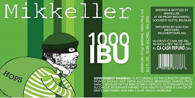
Healthy Spirits: Mikkeller 1000 IBU and more!!!

The newness.

1. Mikkeller 1000 IBU
2. Mikkeller Black Hole Imp. Coffee Stout
3. Uerige Doppel-Sticke
4. Haandbryggeriet Norwegian Wood is back!
5. Nogne-O Imperial Dunkelwit
6. Ommegang Belgian Pale Ale (Dry-hopped)
7. Schneider Brooklyner Hopfen-Weisse is back!
8. Alaskan Raspberry Wheat (Silver Medal Winner GABF 2008-Frut Beer Category)




cheers,

dave hauslein
beer manager
415-255-0610

Blood glucose variations in normal individuals: A chaotic mess

I love statistics. But statistics is the science that will tell you that each person in a group of 20 people ate half a chicken per week over six months, until you realize that 10 died because they ate nothing while the other 10 ate a full chicken every week.

Statistics is the science that will tell you that there is an “association” between these two variables: my weight from 1 to 20 years of age, and the price of gasoline during that period. These two variables are indeed highly correlated, by neither has influenced the other in any way.

This is why I often like to see the underlying numbers when I am told that such and such health measure on average is this or that, or that this or that disease is associated with elevated consumption of whatever. Statistical results must be interpreted carefully. Lying with statistics is very easy.

A case in point is that of blood glucose variations among normal individuals. Try plotting them on graphs. What do you see? A chaotic mess, even when the individuals are pre-screened to exclude anybody with blood glucose abnormalities that would even hint at pre-diabetes. You see wild fluctuations that, while not going up to levels like 200 mg/dl, are much less predictable than many people are told they should be.

Blood glucose levels are influenced by so many factors (Elliott & Elliott, 2009) that I would be surprised if they were as smooth as those in graphs that are frequently used to show how blood glucose is supposed to vary in healthy individuals. Often we see a flat line up until the time of a meal, when the line curves up rapidly and then goes down quickly. It usually peaks at around 140 mg/dl, dropping well below 120 mg/dl after 2 hours.

Those smooth graphs are usually obtained through algorithms that have statistical methods at their core. The algorithms are designed to generate a smooth representations of scattered or disorganized data points. A little bit like the algorithms in software tools that plot best-fit regression curves passing through scattered points (e.g., warppls.com).

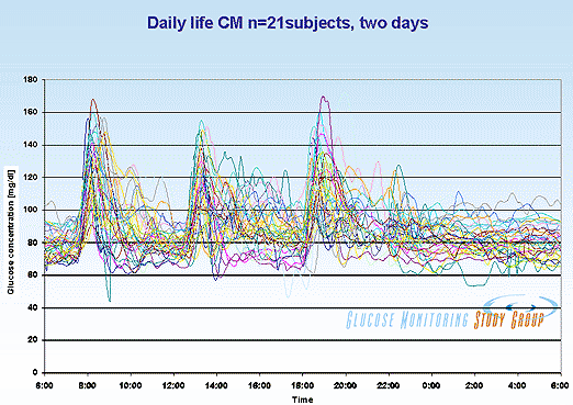
The picture below (click on it to enlarge) is from a 2006 symposium presentation by Prof. J.S. Christiansen, who is a widely cited diabetes researcher. The whole presentation is available from: www.diabetes-symposium.org. It shows the blood glucose variations of 21 young and normal individuals, based on data collected over a period of 2 days. Each individual is represented by a different color. The points on each curve are actually averages of two blood glucose measurements; the original measurements themselves vary even more chaotically.

As you can see from the picture above, each individual has a unique set of responses to main meals, which are represented by the three main blood glucose peaks. Overall, blood glucose levels vary from about 50 to 170 mg/dl, and in several cases remain above 120 mg/dl after 2 hours since a large meal. They vary somewhat chaotically during the night as well, often getting up to around 110 mg/dl.

And these are only 21 individuals, not 100 or 1000. Again, these individuals were all normal (i.e., normoglycemic, in medical research parlance), with an average glycated hemoglobin (HbA1c) of 5 percent, and a range of variation of HbA1c of 4.3 to 5.4 percent.

We can safely assume that these individuals were not on a low carbohydrate diet. The spikes in blood glucose after meals suggest that they were eating foods loaded with refined carbohydrates and/or sugars, particularly for breakfast. So, we can also safely assume that they were somewhat "desensitized" (in terms of glucose response) to those types of foods. Someone who had been on a low carbohydrate diet for a while, and who would thus be more sensitive, would have had even wilder blood glucose variations in response to the same meals.

Many people measure their glucose levels throughout the day with portable glucometers, and quite a few are likely to self-diagnose as pre-diabetics when they see something that they think is a “red flag”. Examples are a blood glucose level peaking at 165 mg/dl, or remaining above 120 mg/dl after 2 hours passed since a meal. Another example is a level of 110 mg/dl when they wake up very early to go to work, after several hours of fasting.

As you can see from the picture above, these “red flag” events do occur in young normoglycemic individuals.

If seeing “red flags” helps people remove refined carbohydrates and sugars from their diet, then fine.

But it may also cause them unnecessary chronic stress, and stress can kill.

Reference:

Elliott, W.H., & Elliott, D.C. (2009). Biochemistry and molecular biology. 4th Edition. New York: NY: Oxford University Press.